One of the most often-asked questions about climate data is, “How long a time period do we need to establish a statistically significant trend?”
Statistical significance of trends is an issue which has been dealt with often at this blog and many others. Yet previous posts, at least here, have made general statements and/or illustrated by example (often with simulated data) how “statistical significance” can come within your grasp or slip through your fingers. But the issue is so important — and so often abused by fake skeptics — that I think it’s worthwhile to give it a close look.
In general terms, the real question we’re considering is: Do these data show a trend? In practical terms the question becomes more specific, usually amounting to: Do these data show a linear trend? In other words, are they reasonably approximated by a pattern over time which follows a straight line, one which is rising (upward trend) or falling (downward trend) but not flat (no trend)?
This is hardly the only trend pattern which can exist, it’s certainly possible for data to follow trends which are not linear. In fact it happens all the time. But establishing the existence of a nonlinear trend is usually harder than showing that a linear trend is present, and a linear trend test will often detect the existence of trends even when they’re highly nonlinear. So, the simple fact is that when scientists study data to determine whether or not a trend is present, the “default” first analysis is to perform linear regression, which is the basic test for the existence of a linear trend.
There are even many varieties of linear regression, but by far the most common is least-squares regression. It has some distinct advantages over other forms (but others have their advantages too), but it’s not our purpose to muse about the virtues and vices of different types of regression. We’ll focus our discussion on the circumstances under which data might or might not reveal the existence of a trend, when we test for a linear trend using least-squares regression.
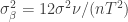
We’ll suppose that we have n data points which represent measurements or estimates of the data values at times which are evenly spaced, e.g., monthly or annual data. The entire time span covered by the data we’ll call T. We recognize that in addition to the underlying pattern (which we’re assuming is linear, but of unknown slope), there’s also noise added into the mix. We’ll say that 

And as I’ve often emphasized, the noise values may not be independent of each other. In particular they may show autocorrelation, meaning that nearby (in time) noise values are correlated with each other. We’ll characterize the impact of autocorrelation by estimating a quantity 
We’ll let 

Note the subscript 

Great! There’s a general formula for you, but what does it mean for real-world data, in particular for global temperature data?
Let’s take monthly average global temperature data from NASA GISS to estimate the parameters. The noise variance is approximately 

Using monthly data, number n of data points in a time span of T years is 
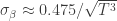
In order to be conservative, I’ll use 0.5 as an approximation for the numerator instead of 0.475, yielding a useful approximate formula for the standard error of the warming rate in NASA GISS monthly global temperature data

That’s the standard error we can expect — but is a slope significant? It will be so at the usual “95% confidence” level if the slope estimate is at least as big as 2 standard errors. Here’s a plot of twice the standard error as a function of the time span T:

I’ve also place a horizontal, thick-dashed line at the value 0.017 deg.C/yr, which is just about the modern rate of global warming. It intercepts our 2-standard-error curve when the time span T is smidgen over 15 years (also indicated by a dashed line).
That means that if we have 15 years of data, we can confirm a trend at the present rate of global warming, right? Not necessarily! When we estimate the slope, our estimate is a random variable. It will approximately follow the normal distribution, with mean value equal to the true slope and standard deviation equal to the standard error. That means that the quantity “estimated slope minus two standard errors” will follow the normal distribution with mean value zero, and standard deviation equal to the standard error. For a warming trend, if that quantity, “estimated minus two standard errors,” is positive, then we achieve statistical significance for a warming trend. If not, then we don’t.
For T just a hair above 15 years, the quantity in question roughly follows the normal distribution with mean value zero because the trend is twice as big as the standard error. So there’s a 50/50 chance of its being above zero and permitting us to declare “statistical significance.” There’s also a 50/50 chance of it’s not being so. Therefore, for the parameters estimated from NASA GISS data, a 15-year time span (actually a wee bit more) gives us about a 50/50 chance to detect a trend with statistical significance. It also gives a 50/50 chance for the significance test to fail — which does not mean there’s no warming (another very common misconception pushed by fake skeptics), just that the given data don’t show it with statistical significance.
How long would we need to have a really good chance — say, a 95% chance — of detecting the trend with statistical significance? For that to happen, the trend has to be four times as large as the standard error. That happens, with the given parameters, when the time span T is 24 years, not 15. Here’s an expanded plot with yet another dashed line indicating a 24-year time span:

So, 15 years of global temperature data from NASA GISS has about a 50/50 chance to show the trend with statistical significance. But for a 95% chance to achieve that threshold, you need about 24 years. All of this is approximate, but it does give a good perspective on the quantity of data needed. It also shows how easy it is for fake skeptics to crow about the lack of statistical significance, even when the trend is present and is real. Would they have the audacity to be so misleading? I’d say that’s something we can expect with 100% confidence.


Loverly.:)
So you mean they have to wait until 2022 before their crowing about no statistically significant warming since 1998 will mean anything?
That certainly won’t work for the instant gratification crowd.
Nice clear explanation as usual Tamino. One small suggestion; I think it would be useful to show how you estimate nu (number of points per effective d.o.f.) or provide a link to an explanation of how to do it.
Is this at all useful?
http://bartonpaullevenson.com/30Years.html
What I’d like to see is the converse argument: is the “absence of warming” statistically significant? E.g.:
Primed reporter: “Has there been statisically significant waming over the last 15 years?”
Climate scientist: “No, but there has been no statisically significant deviation from the previous warming trend either – 15 years is too short to detect a change.”
Would there be much difference in the periods needed to establish confidence in such an end to the warming trend? My guess would be that there’s not much difference but it would be quite sensitive to how you model the previous warming – e.g., the length of time over which the previous slope is taken.
Ed, a simpler & more succinct answer would be as follows:
Climate scientist: “There has been no statistically significant deviation from the ongoing statistically significant warming trend – 15 years is too short to detect a change in the heading of our ship.”
Let’s ask if there is any statistically significant deviation in the relationship between carbon dioxide and global temperature:

No!
very smart the trick ‘2sigma—>4sigma’
[Response: Very common behavior: ‘I don’t understand —> it must be a trick’]
In my bad english,” trick” is admirative. The idea of 4 sigma is very bright and probably original.
It will be interesting to verify that, for all possible 15 years trends(in the monthly set from 1975 to now) approximative 50% are inferior to 2sigma
So, if you tried the same analysis with the time series from Foster&Rahmstorf 2011? My guess is that this would not only decrease the noise, but also reduce the autocorrelation. Would such an analysis be valid in your opinion?
[Response: Yes, it would be valid. And yes, both the noise and the autocorrelation are much reduced.]
But wait… after reading this, how can anyone claim that the warming stopped in 1998 with a straight face, After all that was only 14 years ago…
\sarc
I’m having trouble following this. In particular how you get T3/2…
Are N and n the same thing?
Tamino,
Just noticed the FR 2011 reference and I have been meaning to ask you whether it was possible to replicate your analysis for day time and night time temoperatures??
Never mind – I see where I went wrong (and N and n are the same)
[Response: Yes. My bad … I should have been consistent. Now fixed.]
Tamino: slightly off topic, but the recent Higgs-Boson search aimed for a confidence of 0.000001 (one in a million or so). If physicists want that level of confidence why isn’t the same level adopted elsewhere? Why one in twenty?
[Response: My guess: when you generate as much data as they do you’re going to get some very unusual events simply as a matter of course. So you need to set a higher standard to identify what’s truly “off the scale.” For a better answer, ask the physicists.
As for “why one in twenty?”, it’s because long experience has shown that if the standard is higher you get too many “false alarms” but if the standard is lower you get too many “missed results.” The actual choice (95% confidence) was popularized by the pioneering statistician R. A. Fisher.]
Thomas,
You have to understand the way particle physics data are analyzed. First, you generate an enormous number of interactions. An electronic event trigger automatically selects those events most likely to be of interest (e.g. being particularly high energy and/or having a large amount of momentum perpendicular to the beam axis, which might indicate a decay of a high-mass particle). The trigger itself winnows the events down by many orders of magnitude. Even so, only a tiny fraction of the events saved by the trigger will actually contain particles of interest.
Once you have your sample, you have to figure out a way to discard all the events you don’t care about, so they won’t hide the signal you do care about. You know, roughly what physics your event will have, so you apply “reasonable physical selection principles”–cuts–to the data. When all is said and done, you have applied perhaps a thousand to 10000 different sets of criteria to your data. Now given that you may not even know what mass your “particle” has, you can see where you might generate some spurious “bumps” in your mass histogram. The extra zeros in your required significance are there to guard against such spurious results.
My doctorate was in experimental particle physics.
But wait, according to Stevie Mac, that would make experimental particle physics “unscientific” because they screen their data for validity based on physical principles! I’m so glad Steve has shown us all the way to do science.
It’s worth noting that the global warming trend over the last 3 decades actually is significant at 5+ sigma for the raw surface temperature data and 3+ sigma for the satellite (LT) data (even higher if one uses the Foster/Rahmstorf data adjustment)
And the fact that many different data sources/analyses give a very similar trend (and relatively small uncertainty) allows one to place higher confidence in the trend than if one had obtained the result from only a single data set and analysis.
Of course, one can never rule out the possibility that there might be something that everyone has overlooked, but having multiple independent groups looking and analyzing reduces the likelihood that the indicated warming is only apparent — somehow due to a “systematic error”.
And the likelihood that it’s all a conspiracy is even smaller than that WUWT will start posting real science– which is about as probable as neutrinos travelling faster than light, in Horatio’s humble opinion. (By Dano’s definition, which Horatio subscribes to homheartedly, that is actually not ad hom)
Speaking of which: the OPERA result was doomed by a systematic error. OPERA had LOTS and LOTS of data, which allowed them to claim a “6 sigma” result in the travel time of the neutrinos vs time of travel for light.
But, alas, in the end, all that data was meaningless.
Unfortunately, such a systematic error will throw off the result no matter how much data one has. And any increase in “confidence” obtained by taking more data actually amounts to “false confidence.” OPERA could have taken data until the neutrinos came home (until they could claim a “50 sigma” or even “100 sigma” result ), but it would not have meant a thing if the systematic error remained.
Multiple, independent lines of evidence is the most convincing argument for the reality of climate change.
No matter how climate scientists slice and dice the data (surface temps, lower troposphere temps, arctic sea ice, glacier masses, sea level, atmospheric moisture content, etc), it always seems to come up warming.
That’s very unlikely to be due to either a statistical fluke OR systematic error.
Isn’t the answer simply, because they can? Climate scientists would love to have enough data to make 5-sigma determinations. But they don’t. But the particle physicists do (at great expense, but it’s doable.)
Not exactly. In LHC 5 sigma (0.00000057) was limit requred to announce that Higgs Boson has specific mass, but only 2 sigma (0.05) was limit required to announce that Higgs boson DOES NOT have a specific mass (limit to exclude possibility of existance of Higgs boson with a specific mass).
Confidence is not always what it’s cracked up to be.
A 2-sigma confidence result that is in keeping with well established physics can mean much more than a 5- (or even 6-) sigma result that (supposedly) turns physics on its head (eg: “superluminal” neutrino’s)
Horatio has more “confidence” that Elvis will suddenly appear in the room and sing “The Day Denial Died” than that neutrinos (or any other particles) will be found to travel faster than light.
Can you give a reference or link to the calculation of nu? I’m wondering if it only includes lag-1 autocorrelation, or higher lags as well. (The higher order lag ACs can also be large.) Thanks.
[Response: It depends on the process the noise follows. See Foster & Rahmstorf (2011) for the method used in this case.]
David, there is no way I would give you a million to one odds on any single 5 sigma result in particle physics–including (maybe especially) my thesis result.
I like to think of ANY linear trend merely as first estimate of low-frequency variability that cannot be resolved with the limited record length. For example, a statistically significant trend from a 25-year long record to me indicated the potential of a substantial oscillation at 50-year or longer time scale. For example, I find substantial and significant warming over northern Greenland and Canada from 1987-2010 that are spatially coherent, but the value of this warming trend is time dependent, that is, the longer the record, the smaller the warming, all highly significant, all indicative of accelerated warming … or is possible, that the longer records resolve low-frequency variability (decades to centuries) that become linear trends for shorter records?
[Response: There’s more to global temperature than statistics. There’s also the laws of physics. They tell us, quite unambiguously, that the present trend is not due to some low-frequency oscillation. Even restricting to statistics, there are much longer data series from paleoclimate reconstructions — again indicating that no, it’s not due to some low-frequency oscillation.]
Uh, dude, you’re not really trying to say there’s a 50 year period based on half a period of data, are you?
No, but with 25 years of data and statistics alone, you are hard-pressed to distinguish between the a linear trend and an oscillations that is more than twice your record length … and I totally agree with Tamino, that it is the physics that determine what is happening, not mere trends and statistics. The physics, however, are more complex and non-linear to be described by linear regressions and correlations.
There is more than 25 years of data. What Tamino showed us here is that it takes at least 24 years or more, but not less (I think this is the key point of this blog entry) to determine or reject linear trend from noisy data.
The problem with your reasoning is that you can always reproduce smooth curve at a given interval as a sum of waves (If I remember correctly, this is what Fourier did). Or even, the long enough sine wave (like 1000 or couple of 1000 years) would be almost linear at period of 30 or 100 years – you can always find good match. The problem with this reasoning is that you cannot make any conclusions about such a cycles, as you do not have data available to do any comarison.
On the other hand, if you know radiative properties of earth’s atmosphere (and they are known), you can be quite certain that the temperature will change, if there is a way to block outgoing radiation.
I agree with the sentiment, but would not use the word “unambigiously” as there are many aspects of the physics we understand only poorly. The interaction of ice, ocean, and glaciers around Greenland and Antarctic serves as one (of many) examples. Preponderance of the evidence supports a warming signal embedded within much larger noise of more dominant process I feel.
@Thomas – in Particle Physics, there’s the so called “look elsewhere” effect, if you are looking at a signal in 20 positions, there’s a high likelyhood that you’ll find a 2-sigma signal in there even if it isn’t real (because a 2-sigma signal is expected to be found in 1 out every 20 measurements even if there is no actual signal.)
Since in Particle physics, the scientists are looking in many many more “positions” even than this, the “measured” significance standard of the signal needs to be very much larger.
You could also look at it this way: the scientists are not able to accurately measure the whole “uncertainty” of their measurements, only the part they know about – they know they don’t know, so they know they are significantly *under*estimating their uncertainty, but they have no exact way of compensating for that, except by requiring a much higher standard (5 sigma) so they can be certain the “unknowns” are not causing the signal.
This is very different from for example climate change, where the uncertainty cannot contain that much additional, completely unknown uncertainty, simply because there are no physical mechanisms for this additional uncertainty to be present.
If you want to check this for yourself, I coded up Tamino’s method from F&R2011 as a Javascript tool here. As well as calculating trends and uncertainties, it’ll given you ν and σβ (at the bottom – note these are always in C/year, while the headline figures default to C/decade). Note that you get different ν values for different temperature records – the satellites are very different. Under advanced options you can change the period for calculating ν.
Here are 2σ values of the trend uncertainty over some 15 year periods:
1975-1990 0.158
1980-1995 0.163
1985-2000 0.170
1990-2005 0.169
1995-2010 0.147
Tamino is right that climate is not about merely statisticizing climate data. How much oxygen does anyone really need, on average, over a 24 hr. period? Try switching O2 for CO for a minute. Some thresholds are spikey.
Ahhh, this post illuminates a pernickety issue in the climate debates. Just what I’ve been looking for. Thanks, Tamino.
BPL, that’s a great post on it, too.
Thanks, Barry
I quite like your explanation, Tamino — clear and with lots of generally applicable principles. But it’s still not fully applicable to the fake skeptics, is it? I mean, it applies to a random set of data with a random start point. But fake skeptics like to cherry pick their start points (and their data source) to minimize warming. I would think this shifts the 50/50 and 95% detection probabilities to a somewhat longer time series. Or perhaps that’s not so important because autocorrelation is less than a year?
Statistics is an essential and effective tool in the service of honest Science, it is dangerous when used by liars.
The subject of the current discussion regarding x number of years to establish a statistically significant trend will be misused by the liars.
When one molecule of Carbon Dioxide is added to the atmosphere, there is one molecules effect on the climate immediately.
As the climate system is quite complex the climate change response to increase Carbon dioxide is quite chaotic (not random). As the energy in the climate system increases, there are many factors that will cause temperatures to rise and fall. For example the extra energy may initiate the increase of the turnover of the cold deep ocean water for a while, maybe some more cloud will be generated. It is analogous to the response to the change in seasons, going from winter to summer we don’t get a consistent increase in temperature, we can still get cool and hot days, weeks and even months.
What needs to be made clear is that although there may be x number of years to needed establish a statistically significant trend, we can still confidently say that this days record temperature is most likely due to the increase in Carbon dioxide, and the more maximum temperature records set, the more confident we can be.
Sadly many people can be easily fooled, if it were not the case, magicians and liars could not make a living.
I wanted to wade into this discussion earlier, but found it too dense for my old mind.
Simpler to utter, “This is the end of history”. It is the end when history no longer predicts the future.
Quick question. Talking to a denier lately and they latched onto the line “When the number of data values is not too small”. I’m afraid I’m not at all experienced with statistics. With the noise and short term variations in the temperature how many data points would be considered too small?
[Response: That’s another of those questions which requires work of those who aspire for more than just an off-the-cuff answer. But for some perspective, try here.]
You linked to the page I was asking about, Tamino. Did you mean this post
http://bartonpaullevenson.com/30Years.html
Cheers
Out of interest, and pertinent to these calculations, the following paper in Geophysical Research Letters concludes you need at least 17 years. Enitirely consistent with Taminos analysis
http://www.agu.org/pubs/crossref/2011/2011JD016263.shtml
JOURNAL OF GEOPHYSICAL RESEARCH, VOL. 116, D22105, 19 PP., 2011
doi:10.1029/2011JD016263
Separating signal and noise in atmospheric temperature changes: The importance of timescale
Key Points
• Models run with human forcing can produce 10-year periods with little warming
• S/N ratios for tropospheric temp. are ∼1 for 10-yr trends, ∼4 for 32-yr trends
• Trends >17 yrs are required for identifying human effects on tropospheric temp
Tamino: Can you suggest some reading material on how the “true” uncertainty of a linear trend slope depends on all the autocorrelations in the data?
Specifically, I’ve been looking at the UAH global LT anomalies:
http://vortex.nsstc.uah.edu/data/msu/t2lt/uahncdc.lt
There is a lot of autocorrelation! (I’m guessing this will be true for the other temperature datasets as well.) Calculation the lag-k autocorrelation coefficients r_k, I find that they are large even for high k’s:
r_1=0.85
r_2=0.79
r_3=0.71
r_4=0.66
r_5=0.62
r_6=0.58
etc.
r_12=0.34, and so on.
Isn’t the critical level of correlation for 95% significance given by r_0.95=2/sqrt(N), where N is the number of data points? For the UAH LT dataset N=402, so r_0.95=0.10.
So there is a huge amount of significant autocorrelation, even at relatively large lags where k is beyond 12. There is a lot of inertia in the climate system.
My question is: if k_max is the largest significant lag, how is the uncertainty in the linear trend modified? For example, for lag-1 autocorrelation, Tom Wigley’s chapter “Statistical Issues Regarding Trends”
Click to access sap1-1-draft3-appA.pdf
equation (9) says that the effective sample size N_eff will be
N_eff = N*(1-r_1)/(1+r_1)
so N_eff=33 in my example above. That, in turn, is used to calculate the uncertainty in the slope of the trend via his equations (8) and (5).
But what about the higher lags? I’d like to know how they all add up to give the “true” variance of the slope. I’m wondering if the “true” variance of the slope, when there is a lot of autocorrelation, isn’t so large as to be essentially useless.
Do you know of a paper or textbook that discusses this? Thanks.
Oh, darn. Perhaps this is the Appendix of your Env Res Lett paper with Rahmstorf?
Me again. I should have read that Appendix more carefully first. But when I first read your paper I didn’t have this question in mind, and it’s only today that I realized how how the k>1 correlation coefficients are and how relevant the question is. So perhaps you should just delete my earlier comments. Thanks.
Is there a simple relationship between the autocorrelation functions (at a given lag) of the residuals and the ACF of the values (in this case, the temperature anomalies) themselves?