
From time to time it is suggested that ordinary least squares, a.k.a. “OLS,” is inappropriate for some particular trend analysis. Sometimes this is a “word to the wise” because OLS actually is inappropriate (or at least, inferior to other choices). Sometimes (in tamino’s humble opinion) this is because an individual has seen situations in which OLS performs poorly, and is sufficiently impressed by robust regression as a substitute, to form the faulty opinion that it’s superior to OLS generally. For the record, this comment is not one of those cases.
In reality, OLS is the workhorse of trend analysis and there are very good reasons for that. It’s founded on some very simple, and very common, assumptions about the data, and if those assumptions hold true, OLS is the best method for linear trend detection and estimation. It can be dangerous to use the word “best” in a statistical analysis, but in this case I feel justified in doing so.
Of course that raises some nontrivial questions. What are those assumptions? When might they not hold true? How could we tell? What should we do if we can establish that the OLS assumptions aren’t valid?
Let’s consider the case of linear regression, in which we have a set of 


where 

We can always try lots and lots of values for the parameters, then choose the values that give us the “best” fit. That’s a terribly inefficient way to fit a line to data, but — it actually works! Yet it still requires a way to decide which possible line is “best.” And that can be very tricky indeed!
There is a sensible way — choose the line which gives the maximum likelihood of the observed data. We could even call this “maximum likelihood regression.” But now we have yet another problem: how do we compute the likelihood?
To do so, we have to have a model for the data, and that model must include the behavior of the noise, not just of the underlying signal. Let’s start with the simplest (or at least, most natural) assumption about the data: that the data really do follow a straight line, with deviations which are zero-mean i.i.d. and follow the normal distribution. In this case our model is

where 

Now we can compute the likelihood of our data, given a model — which means, given the slope
These values are called the residuals for our model, and if our model is correct then they’re equal to the true noise values. The probability density for any particular

The joint probability for all the noise values, often called the likelihood function, is the product of their individual probabilities
The maximum-likelihood solution is that which gives the maximum probability.
It’s generally easier to work with the log-likelihood, which is just the logarithm of the likelihood function
![\Lambda = \sum_j \Bigl [ - \epsilon_j^2 / (2\sigma^2) - \ln(\sigma) - \frac{1}{2} \ln(2 \pi) \Bigr ]](https://s0.wp.com/latex.php?latex=%5CLambda+%3D+%5Csum_j+%5CBigl+%5B+-+%5Cepsilon_j%5E2+%2F+%282%5Csigma%5E2%29+-+%5Cln%28%5Csigma%29+-+%5Cfrac%7B1%7D%7B2%7D+%5Cln%282+%5Cpi%29+%5CBigr+%5D&bg=ffffff&fg=333333&s=0&c=20201002)
Maximizing the likelihood function is equivalent to maximizing the log-likelihood function. Furthermore, the log-likelihood involves a sum, which is easier to deal with in most contexts than a product.
If we find the values of
![\sum_j \Bigl [ - \epsilon_j^2 / (2\sigma^2) \Bigr ]](https://s0.wp.com/latex.php?latex=%5Csum_j+%5CBigl+%5B+-+%5Cepsilon_j%5E2+%2F+%282%5Csigma%5E2%29+%5CBigr+%5D&bg=ffffff&fg=333333&s=0&c=20201002)
In fact maximizing this quantity with respect to
![\sum_j \Bigl [ - \epsilon_j^2 \Bigr ]](https://s0.wp.com/latex.php?latex=%5Csum_j+%5CBigl+%5B+-+%5Cepsilon_j%5E2+%5CBigr+%5D&bg=ffffff&fg=333333&s=0&c=20201002)
This is the negative of the sum of the squares of the residuals. Maximizing a negative in the same as minimizing a positive, so the solution for the slope and intercept is that which minimizes the sum of squares of the residuals — hence the name “least squares.” Therefore the least-squares solution is the maximum-likelihood solution when the given assumptions hold true.
Now we can begin to appreciate when the ordinary least-squares (OLS) solution might not be optimal, or even appropriate. When the data violate the given assumptions, OLS is not the maximum-likelihood solution. It may not even be a particularly “good” solution (although it usually is).
What assumptions might be violated? The most often-considered case is when the model of the noise isn’t right. For example, we often consider trend analysis when the noise values aren’t independent. In fact temperature data (especially monthly data) exhibit autocorrelation, where values nearby in time are correlated with each other. If they’re correlated, they’re not independent — and the OLS solution is no longer maximum-likelihood. In such a case, the maximum-likelihood solution is given by generalized least squares (GLS). However, it’s usually a lot easier (and nearly as good) to use OLS but apply a correction when computing the uncertainties of the solution.
Another very common case is when the “normal distribution” assumption doesn’t hold. This is often indicated by the presence of outliers, which are noise values which are quite far from the rest of the data. There’s not universal agreement on exactly how to define an outlier, but sometimes they stick out like a sore thumb. Suppose, for instance, you were surveying the annual incomes of 100 people who were all members of “Oprah’s book club” in Chicago. You might find that 99 of the people had a variety of incomes which formed a nice smooth distribution (probably not the normal distribution, but at least reasonably smooth), but the 100th member was Oprah herself — who made fifty million dollars last year (for Oprah, that’s a slow year)! Her income is so different from that of all the other club members that it sticks out like a sore thumb — we would all agree it’s an outlier.
Extreme values — outliers — can have an extreme impact on the result of OLS. Therefore they can change the result dramatically, sometimes even invalidate it, all because the OLS assumptions aren’t correct, the noise does not follow the normal distribution. Identifying such cases can sometimes be tricky. After all, even noise which does follow the normal distribution can show extreme values! In such a case, those extreme values should be retained and OLS is the right way to go. But in some cases (like Oprah’s book club) the normal-distribution assumption is so obviously not right, and the OLS solution is so strongly affected by the outlier, that OLS isn’t just less than optimal, it’s downright untrustworthy.
Such behavior isn’t limited to regression. Suppose, for instance, we simply wanted to know the average income of members of the Chicago branch of Oprah’s book club. The mean (a.k.a. arithmetic average) of the 99% might be $50,000 per year, which wouldn’t set off any alarm bells. But when Oprah is included, the mean increases to over half a million dollars per person per year! That does set off alarm bells — unless we were talking about Mitt Romney’s country club, such a figure is hard to believe.
In such a case it is often useful to compute a statistic which is resistant to the presence of outliers. For the average, for instance, there is such a statistic called the median. It’s the value which falls right in the middle of the probability distribution, so there’s equal chance of a given sample being above or below that value. If the median income of the 99 non-Oprah members is $44,000 per year, then even if we include Oprah the median value may well still be $44,000 per year, and certainly won’t be anywhere near half a million! In this case the median gives a much more realistic portrayal of the typical income of members of the book club. And if the “average” is meant to convey what’s “typical,” then the median succeeds while the mean utterly fails. This is robust statistics in action. It works.
There are also methods for linear regression which are resistant to the presence of outliers, which fall into the category of robust regression. Probably the most common is to find the solution which minimizes the sum of the absolute values of the residuals rather than the sum of their squares. This is the method of least absolute deviations. It is highly resistant to outliers (as long as there aren’t many of them), and in fact the median is the least-absolute-deviation estimate of the center of a distribution (whereas the mean is the least-squared deviation estimate).
Such a strategy can be generalized by choosing some other function than the square (which gives rise to least-squares regression), or the absolute value (which gives rise to least-absolute-deviation regression), for which we will minimize its sum over all values of the residuals. Such functions are called M-estimators. M-estimators need not actually represent the log-likelihood function, although that was the originating idea and is why they’re called “M”-estimators. In fact both the square and the absolute value can be used as M-estimators, so this broad class includes both least-squares and least-absolute-deviation regression, although when least-squares is selected is doesn’t accomplish the usual purpose — to be resistant to outliers. I have occasionally used the Cauchy distribution as an M-estimator because it’s very close to the square when the residual is small, it suppresses outliers very well, and, well, because it’s interesting!
And I should mention non-parametric regression, which makes no assumption whatever about the distribution of the noise and requires no function to minimize. A popular example is the Theil-Sen estimator, which is the median of all the slopes computed from pairs of data points in the sample. It’s strongly resistant to outliers, to cases where the distribution of the noise is highly skewed, and it’s simple to compute. What could be better!
Incidentally, there are other drawbacks to robust regression which might impact whether it’s the appropriate choice for analysis. For one thing, there are situations in which the robust-regression solution is ambiguous. For another, robust regression (and least-absolute-deviation regression specifically) often requires a lot more computation than least-squares regression, for which the exact “best” solution can be directly computed.
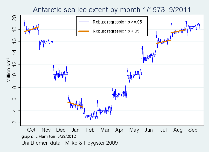
Having indulged in a great deal of general discussion, I’ll finally discuss the context in which this recently came up — sea ice data. Data for the southern hemisphere from the Univ. of Bremen, extending back to 1973, indicate that the very early data include some rather extreme outliers. They’re not so extreme as to invalidate OLS — but they’re extreme enough that it would appear that some form of robust regression is definitely more appropriate. In fact, I don’t have access to that data, but judging visually from the graph I’d guess that it’s straightforward to show that the residuals do not follow the normal distribution and therefore the OLS assumptions do not apply. This definitely calls for robust regression! Or … does it?
Perhaps not. It’s true that the assumptions of OLS do not hold. But, neither do the assumptions behind robust regression. Robust regression is predicated on the model that the data follow a straight line, plus noise which is not normally distributed. If that were true, then the extreme early values would be the result of extreme noise values, but would still represent deviation from a straight-line underlying signal. But what if the underlying signal itself is not a straight line? What if those large deviations aren’t due to noise, but because the signal itself was higher in those earlier years? In that case, the outliers may not indicate non-normal noise, they may indicate that the signal really was higher in those early years, a fact which should reduce the estimated trend rate. But most robust regression methods will treat those values as outlier noise, and they will have negligible (if any!) impact on the estimated trend.
In such a case, which regression method you choose might actually depend on what you’re trying to estimate physically. Let me consider again the incomes of Oprah’s book clube, to make an analogy. If we want to know the “typical” income of a member, then Oprah’s outlier is pretty much irrelevant and should not have undue influence on the result — the median (a robust measure) is definitely appropriate. But if we’re more interested in the spending power of Oprah’s book club, then it would be a capital mistake to downplay the largest value. In that case, the mean — despite it’s non-robust nature and how strongly it’s affected by a single value — is more appropriate.
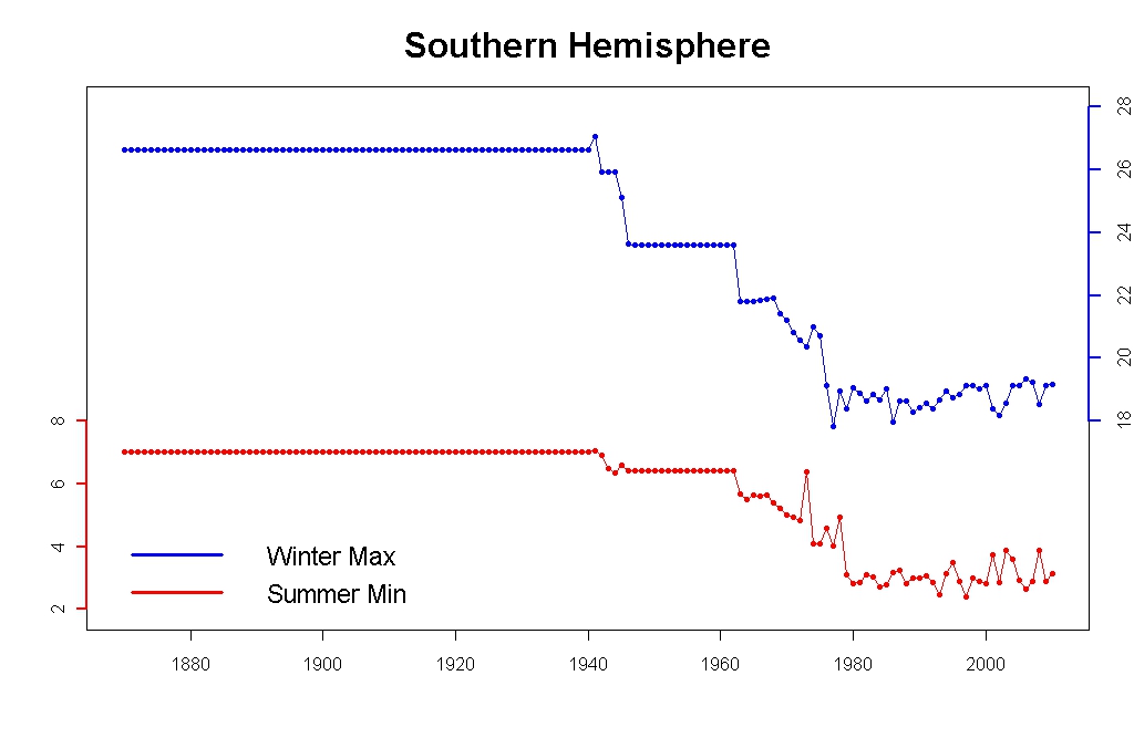
In the case of southern hemisphere sea ice data, estimates prior to 1973 (when the Univ. Bremen data begin) indicate that Antarctic sea ice really was more extensive prior to the satellite era, and the sharp decline indicated by the earliest Univ. Bremen data is part of the actual trend. In that case, if we’re using the Univ. Bremen data to look for the long-term trend, the I submit it may be more logical to apply OLS because it gives full weight to the earliest data, whose extreme values represent the signal, not the noise.
If, on the other hand, we’re more interested in just the recent trend — then those earliest values are evidently out of line compared to what followed. In that case, it might indeed be a better idea to use robust regression so they don’t have undue influence on the estimated trend.
It’s also good to keep in mind that sea ice data for the southern hemisphere since 1973 is demonstrably not following a straight line. In fact the northern hemisphere sea ice data show demonstrable departure from a straight line in the last decade. Treating those departures as “outliers” and substituting robust regression for OLS would be, in my opinion, a mistake. A vastly better approach is to treat the trend as nonlinear.
That doesn’t mean a straight line isn’t a useful model! And it doesn’t invalidate linear regression (OLS or robust) as a useful tool to measure the size of the trend. But it should not be forgotten that, because the signal itself is not linear, robust regression is not automatically a better choice for trend analysis of sea ice, southern or northern.


The thing which strikes me about the whole of this, very useful, discussion of regression methods is that there is little real discussion of the ‘straight line trend’ assumption. If the statement that Antarctic sea ice was greater before the satellite era is correct then perhaps we need a non-linear model (ie one in which d/dt is not constant).
Perhaps (possible niaive suggestion alert) using linear models on slices of the data to obtain a direction field and seeing what happend as the slices get smaller would be a good starting point?
Isn’t that what LOESS is all about?
Tamino seems to like that filter.
So it is…
Honestly hadn’t heard of it before!! And there’s a routine for it in my favourite stats package (R)!!
**Hits self on head severla times**
Wouldn’t loess cloud matters, being so dusty?
For sea ice, the exciting date is 1979 (actually late 1978) when SSMI satellites came in. There is another period of ESMR (73-76???), which is qualitatively different. RMG has a discussion of that in the context of the arctic: http://moregrumbinescience.blogspot.co.uk/2012/03/tempest-in-ice-pot.html
The important point is that its not possible to analyse the sea ice, prior to 1979, without knowing it is a non-homogeneous series and taking that into account, and knowing how the series has been built.
Good stuff. It’s interesting to read about the ideas behind regression, instead of just methods for how to do it. Of course, you didn’t mention Friedrich Gauss!
nice post, many thanks Tamino. Concerning the outliers, I tend to have the following pragmatic (and cynical) reasoning :
– I want to see the general behaviour, and thus I choose the least square
– I was hoping for the outlier to happen, and thus I choose something else :]
In the end, as you said, there is no good trend analysis without a clear model in mind behind (since this can in my mind be considered as an overdetermined inversion)
The data from 1973 is presented in the IPCC Tar fig 2.16 and I think gives a reference to the source.
Even if you use all caps?
I certainly agree that when the data show a clear nonlinear pattern, like September Arctic sea ice, any linear model is probably answering the wrong question. And that outliers are not automatically bad, they might even be the most informative observations, so downweighting them is not always the right choice.
Still, let me put in a few words about what robust regression *is* good for.
* Whether a relationship is nonlinear, and whether outliers are good or bad, might be clear some of the time but other times it’s not. For example, with the October ice extent in my graph, the 1973 value by itself pulls the OLS slope down about 1.26 standard errors (dfbetas). Should I let it? I dunno, that’s what made robust attractive here. The robust line gives a visibly better summary for the upward trend of the other 38 years, accomplishing a reasonable goal since we’re not extrapolating beyond this time period. That high 1973 value does bring up the importance of more information: is it an odd measurement or year, or sign of a substantial nonlinear change? These data by themselves can’t resolve that, maybe other sources can help.
* Robust regression is very easy and not really slow, unless you’ve got convergence problems or massive data. For the Antarctic ice example I cited, robust regression took ~20 times more crunching than OLS, but even on my $299 e-book that’s about one more sip of coffee. I often run both OLS and robust versions of a model, take a quick look and see if they’re much different. If they are, yellow flag. I should slow down to figure out why. If not different, a minor green flag. Not definitive but there’s no sign of outlier/normality troubles yet. In this way robust regression makes a useful and fairly routine part of the toolkit, and sometimes (as IMO with the UB Antarctic data) it provides better summaries.
[Response: Seems like a very reasonable approach to me.]
and …
* As Tamino well explains, OLS is one thing but robust regression refers to many different methods, with different aims and properties. The method I like is an M-estimator based on iteratively reweighted least squares, on each cycle smoothly downweighting observations with large residuals and then re-estimating until there’s not much change. By default it’s tuned to be 95% as efficient as OLS when applied to normally-distributed errors, so with best-case data it still works pretty well. When error distributions have heavier-than-normal tails (outlier prone), however, OLS breaks down quickly while robust regression does not.
Or in one-sample terms, robust regression has a better chance to give reasonable results even when your y variable contains occasional wild errors, whereas OLS has low resistance to those.
Horatio,
“It can be dangerous to use the word “best” in a statistical analysis,
Even if you use all caps?”
Reminds me of a nifty lecture about the Gauss-Markov Theorem, the take-away being that if errors are i.i.d. then OLS is BLUE:
Best (most efficient)
Linear
Unbiased
Estimator
tamino – Thanks for this tutorial.
The discussion of outliers reminds me of another subject worthy of such a tutorial: extreme value theory. You touched upon this some time ago in your post on the Moscow heat wave. In that post you stated:
Fundamental theorems in exreme value theory reveal that in well-behaved cases (which we expect) the distribution of extreme values will follow one of a small number of possible distributions…In fact there are three possible limiting distributions for extreme values.
Intriguing. Further explanation would be appreciated!
I’d like to 2nd that.
I’m interested in the Generalized Pareto distribution;
http://en.wikipedia.org/wiki/Generalized_Pareto_distribution
and peaks over threshold (or POT).
How these extreme value methods might relate to extreme values of water wave heights (in this case deep water rogue waves as these depart from the normally assumed Rayleigh distribution), lake levels (the Great Lakes as an example), river stages (the Mississippi River as an example) and hurricane storm surge events (Atlantic and Gulf coasts as an example).
A friend of mine has been working on Great Lakes datasets, while I’ve spent quite a bit of time looking at long term Mississippi River stage data (cribbing off of his rather vague pointers to the GPD and POT, and not being very satisfied with my results to date).
Also with respect to non-stationary behaviors (or how best to account for trends in these time series, in other words, how trends will change the p-values over time (perhaps just a linear/moving superpositioning of a stationary PDF?).
Anyways very interested in extreme value theory which do/don’t include trends.
Tamino,
I think I mentioned before that I’ve used a metric to compare two distributions that is the expectation of the square of their logarithmic distance. This is closely related to the K-L divergence, and it seems to do a good job fitting both the tails and peak of the distribution.
[Response: Interesting … I’ve researched ways to compare distributions, but never managed to find anything that performs better than the Kolmogorov-Smirnov test (unless you’re comparing observed data to a known distribution, e.g. normal, in which case Shapiro-Wilk is even better).]
A bit off topic, but I’m very curious to know anyone’s expert opinion on the relative merits of the Cramer-von Mises test versus the Kolmogorov-Smirnov test. For whatever reason, I’ve found the CvM test easier to follow and therefore easier to code. But I’m always wondering if I’m losing something.
I think the application also drives the choice of stastical model. For example, if you were trying to predict the total charitable giving of Oprah’s book club members, the median income would do a much worse job of predicting than the average income. But if you trying to predict the increase in charitable giving if 10 new members were added then the median would do a better job.
People with something to sell (denialists, lobbyists, financial companies) will use the model that fits their objective the best. Whereas, scientists and analysts tend to use different models on the same data to try to discern the best predictions.
The biggest problems occur when averages and historical trends are used for planning purposes. Colorado water allocations are based on average flows that were above historical averages*. And we’ve all heard jokes about 401K’s becoming 201K’s or 101K’s.
*H. G. Hidalgo, T. C. Piechota, and J. A. Dracup, 2000: Alternative principal components regression procedures for dentrohydrological reconstructions, Water Resources Research v. 36, p. 3241-3249
Whoowww !!! What a great article. Thank you Tamino, to share your great knowledge with us in such understandable way. This is definitely an article, which I will read many, many times and the one, which will motivate me to learn more. Really, really great thank you !!!
Great post.
OLS has long been the default because it was the easiest by far to implement (and Eli has had to do this on a comptometer). It is the increase in computing power that has brought these better methods to the fore, but even today the EXCEL default trend line has a strong influence, so even letting folk know that there are issues and ways of dealing with them is important.
It would be great if the spreadsheets had a flag: Your data may not be well characterized by simple trend line analysis because:
Glad to see you’re OK!
Hi Tamino! I am wondering about how to reject linearity in data. I’m specifically looking at showing curvature in the MLO CO2 data. The standard procedure I learned was to observe the residuals to look for a pattern in them, but I’ve only done this by eyeball; I’ve never seen any measurement of significance. I’ve looked at a couple options, like curve fitting to the residuals and different chi-squared tests, but I’m still a little uncertain. Any protips?
[Response: Fit a quadratic to the residuals and test for significance.]
If you’re looking at the accumulated co2, then a quadratic fit works well as Tamino has suggested. If you’re looking at the yearly increase, then a linear fit works well as it is the derivative (i.e. rate of change) of the quadratic.
Indeed and indeed!
I was getting thrown because my control residuals were showing significance for a while, albeit much lower significance. I think it was because I was using uniform rather than normal noise; when I switched, the significance went away.
> It would be great if the spreadsheets had a flag: Your data may
> not be well characterized by simple trend line analysis because:
Can y’all suggest
— a reference on what follows ‘because’
— a short checklist of possibilities?
— a suggested way to test for each possibility?
(I’m not assuming such is possible, I’m not the Excel expert in our household — but I’ve heard enough about spreadsheet errors generally to know a lot of handholding needs to go with the tool.
An opportunity presents:
http://www.realclimate.org/index.php/archives/2012/03/extremely-hot/comment-page-4/#comment-232599
I was over at Roy Spencer’s website to take a look at the March temperature readings… and it looks like he’s devised a new skeptic tactic. Temperatures have increased since 1973, BUT….. wait for it, wait for it, population has also increased. Therefore, the two MUST be correlated. The increasing population surely must be causing an urban heat bias in the temperature records. Or maybe it’s all of the CO2 the additional people are exhaling. LOL.
He then applies some sort of ridiculous “correction” factor and eliminates all of the observed warming. All of this in spite of the fact that his own temperature dataset shows a U.S. trend of +0.21C/decade since 1979. He never makes any attempt to demonstrate that there has in fact been any substantial increase in urbanization at any particular site, or more importantly, that any specific site has experienced in increase in UHI contribution. I’m curious as to how the UHI effect is causing decreases in springtime snowcover, increases in surface water temperatures in the Great Lakes and other substantial bodies of waters, lengthening the growing season, making extreme cold more rare, etc. That must be one BIG city.
David F., if there’s been any doubt that Spencer’s left the [science] reservation during the past few years, this new set of posts erases it entirely. It’s really pretty amazing.