Lots of time series, especially in geophysics, exhibit the phenomenon of autocorrelation. This means that not just the signal (if nontrivial signal is present), even the noise is more complicated than the simple kind in which each noise value is independent of the others. Specifically, nearby (in time) noise values tend to be correlated, hence the term “autocorrelation.”
When we attempt to estimate a trend (linear or otherwise) from such data, autocorrelation complicates matters. Usually (almost always, in fact) it makes the uncertainty in a trend estimate bigger than it would be under the naive assumption of “white noise” (uncorrelated noise). There are many ways to compensate for this. Probably the most popular is to take a mathematical model of the noise and compute its impact on the trend estimate. We then estimate the parameters of this model, calculate how much it inflates the uncertainty, and base a more realistic uncertainty estimate on that.
Of course this requires us to have a decent model for the noise process. It doesn’t have to be perfect — but if it’s too far off then our uncertainty estimate will be as well. The simplest model is that there’s no autocorrelation at all (white noise), but in many cases we can prove that such a model is not only incorrect, it’s not even close enough to give realistic results. The most common next step is to model the noise as being of type “AR(1)”, but for some time series (like global temperature data) even that isn’t close enough.
There is, however, a simpler method which doesn’t require building a noise model and estimating its parameters. Simply convert the data to averages over some time span. When we do so, it creates a new time series (the series of averages) which also shows autocorrelation, but less than the original data. The longer the time span over which we average, the less the autocorrelation. This does have the drawback of changing the nature of the noise, e.g. if the raw data have AR(1) noise then the averages will no longer be AR(1). But as we average over longer and longer time spans, the level of autocorrelation gets less and less until it gets close enough to zero that we can treat the noise as white noise, at least to a first approximation.
Another drawback is that there are fewer averages than there are original data values. If we average over every 12 data values (say, converting monthly averages to annual averages) we only have 1/12th as many data values. This too decreases the precision of our estimate, even if the noise is already white noise, but by a surprisingly small amount. But the point of averaging over longer and longer time spans isn’t necessarily to get the best estimate of trend uncertainty, it’s to get a rough estimate which is nonetheless realistic, and which is easy to compute, especially since almost all of those computer programs which compute trend lines automatically also compute the uncertainty according to a white-noise model.
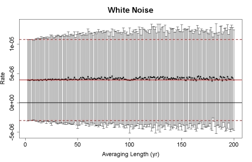
Suppose for instance we start with actual white noise. I generated 10,000 white noise values for a 10,000-year artificial time series with no trend at all, and estimated the linear trend rate and its uncertainty by least-squares regression. Then I computed averages over various time spans, from 2 years to 200 years, to show how the trend estimate and its uncertainty using a white-noise model would change. Here’s the result:
Black dots with error bars show the 95% confidence interval for the trend using a white-noise model for the noise. The solid red line shows the estimate based on all the data, and the dashed red lines show its 95% confidence interval. The solid black line shows the true trend, which of course is zero.
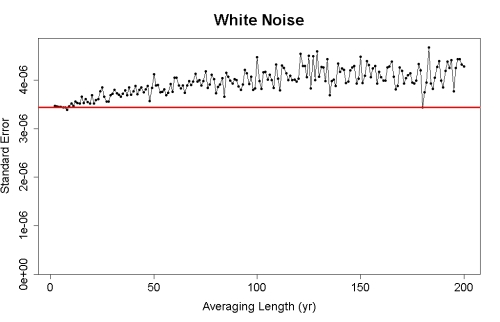
All the estimates are about the same, and all the confidence intervals include the true value. Averaging only inflated the uncertainty slightly, as we can see by graphing the standard errors as a function of averaging length:
Therefore taking averages only slightly degrades the precision of a trend estimate, at least as long as we still have a respectable number of averages. Since my longest averaging span was 200 years and I started with 10,000 years of data, I have at least 50 data values for each choice of averaging length.
Now suppose the data are very strongly autocorrelated. I generated 10,000 data values from an AR(1) noise process with lag-1 autocorrelation set to a whopping 0.99. Now the white-noise uncertainty estimate is not even close to being correct. Nonetheless I compensated for this by modelling the noise as an AR(1) process (the correct model). Then I computed averages over all time spans from 2 to 200 years, estimating the trend and estimating its uncertainty using a white-noise model. Here’s the result:
Again, dots with error bars show the 95% confidence interval for the white-noise model using averages. The solid red line is the estimated trend using all the data and the dashed red lines show the 95% confidence interval corrected for autocorrelation. The solid black line shows the true trend (which of course is zero).
For short averaging intervals, the white-noise uncertainty is too small. In fact for averaging intervals less than about 5 years the 95% confidence interval excludes the true value (zero). But as the averaging interval gets longer and longer, the white-noise confidence interval gets closer to that which is estimated from the original data when corrected for autocorrelation. Averaging over longer and longer time spans has removed most of the impact of autocorrelation on the estimated uncertainty in the trend. It hasn’t removed it all because even at a lag of 200 years the autocorrelation in the original data is still 0.134. But at least we are able to get a realistic appraisal of the trend and its uncertainty, and we can use a white-noise model so we get that straight from a standard statistics program.
It also works for more complex noise models. For instance I generated 10,000 artificial values from an ARMA(1,1) noise process, with autocorrelation which is still quite strong although not as strong as that I used for the AR(1) process. Again I estimated the trend and its uncertainty compensated for autocorrelation. Again I averaged over time spans from 2 to 200 years and estimated, from that, the trend and its uncertainty using a white-noise model Here’s the result:
Once again, as the averaging interval gets longer and longer the white-noise confidence interval gets closer to the autocorrelation-corrected confidence interval.
If you have some time series data to study, and you’re not sure how much autocorrelation might affect a trend estimate or how to compensate for its effect, try averaging over longer and longer time spans and see how the confidence interval changes as you do so. If the confidence intervals seem to converge to a consistent range, this is a decent approximation of the correct range — and you don’t have to use a non-white noise model to get it. In fact you don’t even have to know how the noise behaves to do so.
Do be wary of letting the averaging interval get too long, however. Then you’ll have so few averages that your results will no longer be trustworty. It’s a good idea to have at least 30 values, although you can push the limit until you only have 20 values and see what happens.
Be wary also of those time spans for which the average doesn’t include a complete averaging interval (there may be such spans at the start or end of your data). Leaving them out is probably best, but you could leave them in just to see what happens.
And don’t regard this procedure as the best way to estimate trend uncertainty. It is, however, a rough-and-ready method which can get you in the ballpark.


Probably a stupid question, but what is autocorrelation for annual global temperature data?
Don’t quite understand what you are asking. Look at annualized GISTemp for example. One year is often similar to the prior year. As an example, 2011 and 2012. Enough of that and one has some form of autocorrelation. Indeed, there is enough of that.
From the post: “Now suppose the data are very strongly autocorrelated. I generated 10,000 data values from an AR(1) noise process with lag-1 autocorrelation set to a whopping 0.99. ”
So I guess what I’m asking is, “What is a similar statement that can be made about annual global temperature?”
[Response: The lag-1 autocorrelation of GISS annual average global temperature (after removing nonlinear trend) is about 0.2. However, there’s not a lot of data so that estimate is quite uncertain.]
Nice piece here, and “A shorter version of the animation here.
Explanation: The animation shows observations and two simulations with a climate model which only vary in their particular realisation of the weather, i.e. chaotic variability.”
While I really don’t have the math background to explain it to you, you may want to check you the Kalman filter that the US Navy uses for precision navigation. As someone who was a operator in the navigation center on both Polaris and Poseidon submarines, I found the accuracy of the Kalman filter amazing.
[Response: Kalman filters are great. But they’re not a “black box” where you push in data and answers come out. They require a model — both for how the signal evolves and how the noise behaves. In many cases, the Kalman filter simply reproduces what you’d get from the same model in a different setting.]