Through a Picket Fence

Suppose you’re an astronomer interested in variable stars — stars which change brightness. You decide to collect some data on the brightness of a newly discovered variable. It never gets brighter than magnitude 9, which is too faint to be detected with the naked eye, but you’re at a major observatory so that’s no problem. You have access to, and training in the use of, high-precision CCD photometry so your data will be outstanding. Of course, you can only see it at night and there’s stiff competition for observing time on the observatory telescope, but you manage to schedule regular observations at precisely midnight every 16 days for slightly over a year.

If we graph the data and examine the graph, we might instantly know that we understand its behavior:

Such a graph is called a light curve. By the way, magnitude is an “inverted” scale, for which higher numbers indicate lower brightness, so the numbers on the magnitude axis go from highest at the bottom to lowest on the top. Pretty clearly, the star fluctuates in periodic fashion, repeating the same cycle over and over again (at least, it did while we were watching it). The period is about 80 days according to the graph, which is confirmed by Fourier analysis of the data, showing a strong peak at frequency 0.0125 cycles/day, period 80 days.

Well … there it is. Case solved.

You’re preparing your analysis to be published in the Information Bulletin on Variable Stars when you find, to your dismay, that another observer has beat you to the punch. Not only that, they collected much more data than you did, observing the star at exactly midnight every day. Woe is you! If only you had published faster! But when you look at their light curve, suddenly you’re glad you didn’t publish faster:

Their graph indicates that the period is only 20 days. So does their Fourier spectrum, indicating frequency 0.05 cycle/day (period 20 days):

What the … ???

You go back to your original data and re-compute the Fourier spectrum, but this time, instead of accepting the default settings you instruct it to scan a larger frequency range — one which will include the frequency reported by your competition. In fact you scan a much larger frequency range. You get this:

Sure enough, there’s the peak at frequency 0.05 (period 20), and there’s your original peak at frequency 0.0125 (period 80). There are also peaks at frequencies 0.075, 0.1125, 0.1375, and 0.175 (periods 13.333, 8.889, 7.273, and 5.714). And they’re all the same strength. According to this, the “true” frequency (if there is such a thing) could be any of those values.

In fact the power spectrum looks like a sequence of identical copies of the power spectrum from frequency 0 to 0.03125, laid end-to-end, with odd-numbered copies in normal order and even-numbered copies in reverse order. You email the other observatory and request their data, which they kindly provide, then you Fourier-analyze that with a larger frequency range:

There’s the peak at frequency 0.05 (period 20), but none at 0.0125 (period 80) or those other periods you noticed. But now there are peaks at frequencies 0.95, 1.05, and 1.95 (periods 1.0526, 0.9524, and 0.5128). Could one of those be the “real” frequency? And … what the heck is going on here anyway?

You decide to superimpose your data (plotted in black) with theirs (plotted in red)

Aha! What you’ve observed is the phenomenon called aliasing. They believed the star is fluctuating with frequency 0.05 cycles/day, you believed in fluctuation frequency 0.0125 cycles/day. It turns out that at the times you chose for observation, those two models have exactly the same values — each is an alias of the other. It’s rather like you were looking at the behavior through a “picket fence” of time. The two different fluctuations are quite different when you weren’t looking, but they’re identical when you were.

It arises because you have observed the star at perfectly regular intervals of 16 days — or to put it another way, your data show a sampling frequency of 1/16th observation per day, or 0.0625/day. Suppose the true frequency is f so the light curve is given by

.

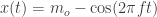
The quantity is the mean magnitude. Suppose also that we observe it at equally spaced times (a case called “even sampling”)

.

Then the data values are

.

Now consider a different fluctuation at frequency . Those data values would be

.

But it’s a fundamental property of the cosine function that it is periodic with period , i.e.,

,

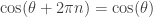
for any number and any integer n. Therefore the new values are

,

i.e., they’re exactly equal to the old values. If the data are only observed at regular intervals, then there’s simply no way to tell the difference between fluctuation at frequency f and that at frequency . If we call the sampling frequency , then there’s no way to tell the difference between fluctuation at frequency f and that at frequency , where n is any integer at all (positive or negative) — they’re all aliases of each other.

Now word arrives that yet a third astronomer at a third observatory has analyzed the spectrum of the star — not the Fourier spectrum, but the optical spectrum (breaking light into its component colors). On that basis, they suggest that the star might be a Cepheid-type variable. Cepheids can have periods as long as 20 days, but they can also have periods as short as a day. Now there’s genuine ambiguity about the period of this star. The once-a-day data indicate the period might be 20 days, or 1.0526, 0.9524, or 0.5128 days. Which is it really?

Fortunately, this star wasn’t just observed by professional astronomers with major observatory telescopes. It was also observed by a host of amateurs, some using small telescopes, some just binoculars. They didn’t apply high-precision CCD photometry, they used visual photometry, comparing the star to nearby stars of known magnitude for a visual estimate of its brightness. Visual data aren’t nearly as precise as CCD photometry. But there’s an army of amateurs worldwide, and they’ve collected a lot more data than the pros. And … more to the point … their observations are not taken at regular time intervals, the amateur data shows uneven sampling. Here’s their data:

It doesn’t look like much — and it’s certainly very noisy. But when we Fourier analyze the data we get this:

It turns out the true frequency is 0.95 cycles/day, and the true period is 1.0526 days.

In the real world, professional astronomers are well aware of the phenomenon of aliasing, they tend not to observe at exactly the same time of night every time, and they rarely take only one observation per night anyway. So, this is just a hypothetical example. But it illustrates the phenomenon of aliasing quite well.

When data are sampled at a regular sampling frequency , the highest frequency about which we can get useful information with Fourier analysis (or other period analysis methods) is half the sampling frequency, known as the Nyquist frequency. If we compute the spectrum at frequencies beyond the Nyquist frequency, we’ll get identical copies, alternating between normal and mirror-image copies, laid end-to-end. We can’t really explore “frequency space” beyond the Nyquist frequency. That’s one of the reasons I encourage amateur astronomers (and professionals too) not to observe at regular intervals, but as much as possible to randomize their times of observation.

Even with uneven sampling we can still have aliasing, if the density of data is periodic. The aliases generally won’t be exact copies of the real signal frequency, only approximately so, and alias peaks in a Fourier spectrum will generally be weaker than the real peak. But if the data density is very strongly periodic, the aliases can be nearly as strong as the real signal, sometimes so much so that it’s not possible to be sure which is real. And unfortunately, some periodicity in data density is unavoidable. You can’t observe most astronomical objects during daytime, so there’s a natural sampling frequency of once per day. Every year the sun travels through the constellations of the zodiac and often obscures our targets, so there’s another natural sampling frequency of once per year. Each of these cycles leads to aliasing in period analysis, but if the observation times are reasonably irregular then the aliasing is usually quite manageable.

Uneven sampling is a solution to the aliasing problem, but it has problems of its own. It alters the behavior of period analysis like Fourier analysis, making it — and its statistical evaluation — more complicated. But much mathematical ingenuity has developed solutions to many, even most, of those problems, so on the whole, in my opinion, uneven time sampling is not the bane it was once thought to be, it’s a great blessing.

It’s also true in the real world that telescope time at major observatories is very hard to come by. And there really is an army of amateur astronomers worldwide who contribute vast amounts of data to our scientific knowledge. Some of them have even mastered the art of high-precision CCD photometry (with the help of not-too-expensive CCD cameras). They are an extraordinarily valuable resource to the astronomical community and have contributed mightily to our understanding of the universe. In fact, some of the most famous astronomers in history had their start as amateur observers. But that is another story …