
Since the subject came up …
There are certain claims (some false) about the correlation (or not) between CO2 in the atmosphere and global temperature. Several folks have pointed out that we shouldn’t really be looking at the correlation between temperature and CO2, but between temperature and CO2 forcing.
This is the climate forcing due to a given concentration of CO2 in the atmosphere, and it turns out to be a logarithmic function of the CO2 concentration. It can be put in many (equivalent) forms, but the one I will choose is
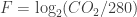
where CO2 is in units of parts per million (ppm) and the climate forcing is in units of doublings of CO2 (that’s why the logarithm is taken to base-2). Note that if the CO2 concentration is 280 (its pre-industrial value) then the climate forcing is zero, so this is the climate forcing due to CO2 concentration relative to pre-industrial.
For CO2 data, I used the yearly averages since 1958 of measurements at the Mauna Loa atmospheric observatory, and from 1880 to 1958 an interpolated dataset from the Law Dome ice core in Antarctica. The CO2 data looks like this:

The climate forcing data look like this:

They certainly look remarkably similar! And so they are, except the numerical values on the y-axis reveal that while CO2 has climbed by over 100 ppm, we are still only a bit above half-way to doubling (on a logarithmic scale). We also see that already in 1880, CO2 climate forcing was a little bit above zero because CO2 was a little bit above pre-industrial.
I started with 1880 because I’m using the global temperature data from NASA:

Now that I’ve selected the data, what do they have to say?
Here’s CO2 climate forcing .vs. global temperature:

The correlation coefficient between the two variables is a whopping 0.9467, but what really counts is its statistical significance (which is not guaranteed by a large coefficient). In this case the significance is undeniable (with a p-value < 10-15).
Perhaps most notable is the slope of the correlation. That’s why I chose units of “doublings of CO2” for the climate forcing: because this slope is an estimate of the climate sensitivity, the amount of global warming (relative to pre-industrial) we expect from a doubling of CO2 (relative to pre-industrial).
That value (2.4 deg.C per doubling) is close to the mean of what the climate models have to say.
This blog is made possible by readers like you; join others by donating at My Wee Dragon.


Wow, just wow. I felt that in my guts (and had some experiences from the time I modelled microchip packaging heat flows with finite elements), but I wouldn’t have expected this to be so clear cut. Many thanks for taking up the idea and throwing your expertise at it!
Still the wobbles on the lower end should make us curious. A data acquisition problem?
Concerning the climate sensitivity, this is the “short term climate sensitivity”, the “left end” of the ΔT(F,t) – function. There is also an “equilibrium climate sensitivity”, which is the asymptotic limit for t → ∞, which is clearly higher (or is it? and how much?).
That 2.4 deg.C would be the Transient Climate Response.
The IPCC suggests TCR likely lies between 1 °C and 2.5 °C doubling and an Equilibrium Climate Sensitivity 2.5°C to 4°C.
To my understanding your estimate of TCS would support an ECS closer to 4C.
I’m wondering if the (longish) period selected might account for some lag in the climate system, putting the result somewhere between TCR and ECS.
barry,
If you run the regression for a shorter period (say 1970-to-date) you get the same number so using the result.
An assumption in using this ‘same number’ to calculate TCR is whether or not the CO2 increase (or more precisely ‘forcing’) is running at the level expected in the TCR analyses. And this of CO2 alone isn’t the case. The NOAA AGGI shows CO2 forcing 1979-2020 running below the +0.037Wm^-2/yr increase. The annual CO2 forcing has been slowly rising through this period, from +0.025Wm^-2/yr to +0.032Wm^-2/yr, ever below the forcing anticipated by TCR.
But CO2 is not the only forcing at work. The NOAA AGGI data suggests CO2 is roughly 80% of the total (positive & negative) forcings (natural & anthropogenic) which would give a back-of-envelop number for AGW as a whole to be running at +0.031Wm^-2/yr to +0.040Wm^2/yr.
I think the problem with nailing-down a precise ECS value is that there are long-term effects a forcing imposes on the climate which make a significant impact on the final value while our usable climate data does not stretch that far. There are folk who say ECS can be calculated by simply subtracting the TOA energy imbalance to provide the amount of AGW forcing so far converted into AGW. Their results yield a low ECS at the bottom end of the IPCC range. But such analyses assume it is all about energy smoothly heating up the world, an assumption which is smoothing over some rather meaty physics.
It seems that the change in slope happens quite remarkably when there is a change in the method to measure CO2 concentration. Is it possible to have the same method for the whole period? What happened around 1960 so that the temperature anomaly seems to change slope? Can we explain this other than the CO2 concentration?
Dom,
“Is it possible to have the same method for the whole period?”
That “change in slope” is found in the ice core data (as shown here which graphs CO2 records … derived from three ice cores obtained at Law Dome, East Antarctica from 1987 to 1993.”) The post-1959 ice core data is a good match to the record derived from atmospheric sampling (in 1978 Law Dome giving 333.7ppm & MLO 334.51ppm). So there may be a remarkable coincidence that CO2 ramped up just as Keeling began his CO2 measuring but it is just a coincidence.
In hindsight (20/20 as usual), it is not surprising that F tracks CO2 so well. Log(1+x) is approximately x for x < 1. Here, the increase in CO2 is x. Thus F should be proportional to the increase in CO2 (for "small" increases in CO2). It is nevertheless good to see the correlation for the exact F, and as Tamino notes, the correlation with F has a nice interpretation.
Berkeley Earth publishes uncertainties in its annual temperature file. The uncertainties are large in the 19th century and unusually large in the early 1940’s.
Tamino
This is of course off topic: it was no longer possible to add a comment to your last thread in February dealing with sea levels.
A few weeks ago, Andy May wrote three consecutive threads about sea levels. In the third one
AR6 and Sea Level, Part 3, A Statistically Valid Forecast
he posted some statistical stuff based on a small R program.
My stats and R skills are pretty minimal, so I’d appreciate it if you’d take a closer look at what he posted there.
Thanks in advance for helping.
Really nice analysis! And it’s worth noting that your result (2.4 K) is basically identical to Manabe & Wetherald (1967), 55 years ago, using the first-ever computational climate model. They found a 2.36 K increase in T for doubling of CO2 from 300 to 600 ppm.
We knew enough 55 years ago to act. Time to stop stalling and get to work.
Some things just refuse to change.
1. A chart of log2(CO2equivalent/278) vs. Temp. anomaly would be a useful addition to account for increases in methane, N20, CFC etc. And if you are in the mood throw in Land use and sea ice albedo change to get a pretty good estimate of TCR.
2. What is the assumed lag between TCR and ECS? My understanding is that it takes about 10 years (as per Ken Caldeira) to see about half of the forcing manifested in NASA GISS global average surface temperature, about 30 years to see about 75%, and 100 years or more to asymptotically approach ECS.
3. Recent article by Hausfather et al. on Carbon Brief https://www.carbonbrief.org/guest-post-how-climate-scientists-should-handle-hot-models and in Nature summarizes recent ECS estimates, with IPCC estimate at 2.5-4.0 C.
Glen Koehler,
The inclusion of other forcings would drop any TCR calculated from solely CO2 forcing down by 17% (so in this case 2.4 x 0.83 = 2.0) as CO2 roughly comprises 83% of total net forcings (as listed in IPCC AR5 WG1 AII Table 1.2).
The main difficulty with using annual forcing & annual temperature to calculate TCR is the big short-lived negative volcanic forcings which do not have time to ‘heat soak’ the planet yet do upset the TOA energy balance. To handle this properly would require more of a model than a simple regression of forcing v temps.
But as a simplistic alternative, accounting for only 25% of the volcanic forcing yields the graphic posted on this page on 4th May 2022 which shows the wobbles when all forcings are accounted closely follow the smoother CO2 forcing curve.
Thanks Al. So the CO2 vs. Temp. anomaly regression is assigning warming to CO2 that was due to other causes, which a TCR calculation for CO2 alone should not do.
Using KiwiGriff’s ratio of ECS/TCR at roughly 1.67 (from the 4.0/2.4 example), then a CO2-only TCR of ~2.0 gives a CO2-only ECS of ~3.3C. Which is near the exact center of the IPCC AR6 range of 2.5-4. And almost exactly matches the 3.4C ECS value predicted by Andrew Dressler a few years ago.
The recent 10-15 year average annual warming rate trends at https://sites.google.com/site/housman100resultstemperarypost/cited-graphs are 0.3 to 0.4C per decade. That lines up with a recent James Hansen speculation about a possible warming acceleration for the next few decades due to (if I remember correctly) aerosol reduction as fossil fuel use declines (and possibly also due to ocean CO2 sink saturation?).
At those rates of increase, the equilibrium temperature for the Arctic Ocean to be essentially ice-free in late summer, and for the Greenland ice sheet melt to become self-propelled (i.e. unstoppable) — both of which have been estimated at about +1.7 C over preindustrial vs. current +1.2C — will be reached in only 15-20 years. What a sad legacy for my Baby Boomer generation to leave. I hope we can turn this battleship around.
Good to see Tamino back in action. That’s a start! I would love to see Tamino debunk Cliff Mass’ “What, me worry?” blog posts. IMHO the harm Cliff does by using his reputation and large audience platform to dismiss climate disruption is incalculable.
That graphic showing GISTEMP linear trends for various length of time periods was produced to demonstrate that any analysis considering a record less than 20-years yields results that wobble above and below a more reliable measure and to dismiss statements asserting it was currently sky-high (+0.5ºC/decade which was based on an Ecological Economist mis-speaking).
Given that, I’d suggest the graphic is showing the current rate of warming is likely below +0.3ºC/decade and unlikely in the range “0.3 to 0.4C per decade.”
The rate of warming was firmly set at roughly +0.17ºC/decade until ten years ago so there is certainly acceleration. But to suggest it has reached above +0.3ºC/decade is making too many assumptions for me.
I wouldn’t rule out future acceleration that would then push warming above +0.3ºC/decade. In particular, you mention the drop in SO2 emissions as coal is phased out and that is a worry. But that is for the future not the here-&-now.
RE Cliff Mass: “My Views on Climate Change/Global Warming”
April 16, 2022.
https://cliffmass.blogspot.com/2022/04/my-views-on-climate-changeglobal.html.
– No need for emergency response if the Mass conclusions are true.
– If they are not true, then the already-difficult challenge to mobilize a societal response to reduce global greenhouse gas emissions by 50% over the next 10 years, and by >95% in 28 years, becomes even more difficult (impossible?) when a prominent trusted authority says there is no emergency to require such action.
Cliff Mass:
“1. Greenhouse gases (such as CO2 and methane) are increasing and human emissions are the main cause of the rise.
2. The planet has warmed about 1°C during the past century and most, but not necessarily all, of that warming is due to increasing greenhouse gases in the atmosphere.
3. Increasingly greenhouse gases affects some extremes (e.g., heat waves), but not others (such as the intensity of winter storms reaching the Northwest)
4. Changes in extremes due to global warming are relatively small today and generally eclipsed by natural variability. Changes in extremes (such as heatwaves) will increase later in the century.
5. Global warming is not an existential threat to mankind but will reduce the rate at which mankind becomes richer.
6. Mankind can make considerable adaptations to climate change, preventing most economic and human impacts.
7. There is great hope for reducing global warming using improved energy technologies (e.g., nuclear energy, renewables, replacing coal/oil with natural gas, better storage technologies) and pulling CO2 out of the atmosphere (sequestration).
8. Improved weather prediction and adaptation efforts have greatly reduced the vulnerability of humanity to global warming effects. Deaths due to extreme weather have declined 95% during the past century.
In short, global warming is a serious, but manageable, problem that should be amenable to technological solutions.is not required.
“1. Greenhouse gases (such as CO2 and methane) are increasing and human emissions are the main cause of the rise.
2. The planet has warmed about 1°C during the past century and most, but not necessarily all, of that warming is due to increasing greenhouse gases in the atmosphere.
3. Increasingly greenhouse gases affects some extremes (e.g., heat waves), but not others (such as the intensity of winter storms reaching the Northwest)
4. Changes in extremes due to global warming are relatively small today and generally eclipsed by natural variability. Changes in extremes (such as heatwaves) will increase later in the century.
5. Global warming is not an existential threat to mankind but will reduce the rate at which mankind becomes richer.
6. Mankind can make considerable adaptations to climate change, preventing most economic and human impacts.
7. There is great hope for reducing global warming using improved energy technologies (e.g., nuclear energy, renewables, replacing coal/oil with natural gas, better storage technologies) and pulling CO2 out of the atmosphere (sequestration).
8. Improved weather prediction and adaptation efforts have greatly reduced the vulnerability of humanity to global warming effects. Deaths due to extreme weather have declined 95% during the past century.
In short, global warming is a serious, but manageable, problem that should be amenable to technological solutions.”
ugh, please remove duplication