Regional Marcott

We’ve already examined the big picture of global temperature according to the recent reconstruction for the holocene (in particular the last 11,300 years) from Marcott et al. We also took a close look at the recent uptick in temperature. Now let’s see about some of the regional differences indicated by these data.

In their supplemental materials, Marcott et al. included the reconstructions restricted to three very wide latitude bands: the northern extratropics (from 30N latitude to the N.Pole), the southern extratropics (from 30S latitude to the S.Pole), and the equatorial band (from 30S to 30N latitude). These reconstructions are computed using their “Standard 5×5” method. But we noted that they may suffer from a difficulty, that as time marches forward, the drop-out of more and more proxies can lead to spurious jumps in the average temperature. This is especially difficult for the most recent time period, because that’s when there are the fewest proxies remaining (so things are less accurate anyway) and there’s more proxy drop-out.

To help with this problem we applied a differencing method rather than a straightforward average. Let’s apply that method to the latitude bands and compare the results with the Marcott et al. standard 5×5 result. We’ll also apply it to a limited sub-region of the northern extratropics which I’ll call the “near north Atlantic” region, covering latitudes 30N and above, longitudes from 90W to 30E.

The Marcott result for the northern extratropics shows two questionable features recently, a pronounced drop followed by a pronounced rise:

The difference method shows neither:

Comparing the two reveals that the recent drop-rise is their main difference (other than the fact that the Marcott result is strongly smoothed due to their Monte Carlo procedure):

The drop defies belief, being more than a full deg.C, and the rise at nearly 2 deg.C is even less plausible:

I conclude that the drop-rise is an artifact of proxy drop-out, but the agreement between the methods for most of the time span argues for correctness during earlier times.

The interesting and useful result is that over the course of the holocene, the northern extraropics shows so much more temperature change than the globe as a whole. Whereas the global temperature covers a range of about 0.7 deg.C, the northern region changes by more than twice that, a bit over 1.5 deg.C. This suggests that perhaps the bulk of global temperature change over the last 11,300 years has been in the northern hemisphere extratropics.

Marcott et al.’s result for the equatorial band actually shows a slight warming over the early holocene, with another large uptick at the very end:

The differencing method shows much less uptick:

Direct comparison illustrates their good agreement except for the uptick at the end:

The southern hemisphere extratropics according to Marcott et al. shows cooling over the early holocene, with yet another large uptick at the end:

The differencing methods shows about the same thing:

Comparison reveals their general agreement, and that the ending uptick by the differencing method is only slightly less than that of the Marcott “standard 5×5” method:

The recent sizable uptick in the southern extratropics is not an artifact of proxy drop-out. However, this region has fewer proxies than the others, and by the time one gets anywhere near the 20th century fewer than 10 proxies remain. This doesn’t entirely invalidate the recent result, but does call it into question. Furthermore, the most recent southern uptick is larger than indicated by instrumental data. For these reasons I regard the recent southern uptick as suggestive, but far from reliable.

We can take the differencing-method results for the three latitude bands and combine them into an area-weighted average for the entire globe:

Then ending uptick is larger than it was in the difference-method estimate simply using all the proxies, as was done in the last post. This is because the uptick is strongest in the southern extratropics which have fewer proxies and are therefore underrepresented in a simple averaging method. Area-weighting compensates for this and gives the southern uptick the weight that its geographic area calls for. But again, the recent uptick is based on far fewer proxies — especially in the south — so I wouldn’t put too much stock in it.

For me, the truly fascinating aspect of this is the strong differences between geographic regions. We can see this most clearly by showing the latitude bands on one graph:

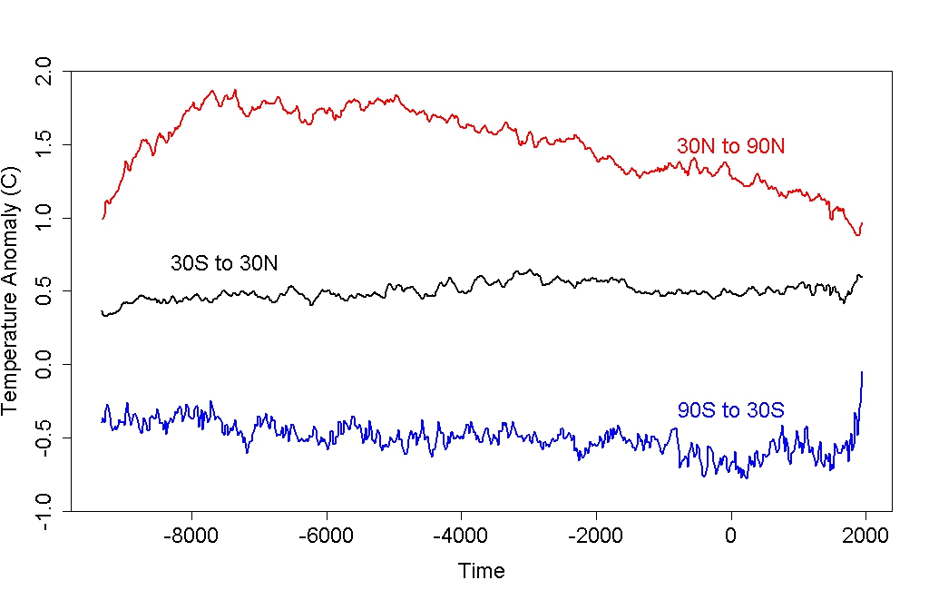
Even on this reduced scale the most important conclusions are apparent. Most of the temperature change throughout the holocene has indeed been in the northern extratropics, with slow and steady cooling the pattern since about 5000 BC. The southern extratropics has cooled early, and by much less than the northern extratropics. The equatorial band showed a slight warming up to about 3000 BC.

As Marcott et al. point out, this pattern of polar cooling and slight equatorial warming is consistent with the change in earth’s obliquity (the tilt of its axis) over time. Obliquity has reduced slightly since about 9000 years ago, which tends to bring less sunlight to polar regions but slightly more to the equator. Its effect has been amplified in the northern rather than southern extratropics, perhaps due to that region’s greater sensitivity to ice and snow albedo because of the much greater amount of snow in the north due to the much greater amount of land in that hemisphere. Another factor amplifying the northern cooling over the southern may be changes in the Atlantic meridional overturning circulation (AMOC).

Marcott et al. also point out the even more exaggerated holocene cooling in the northern hemisphere near the Atlantic ocean. I isolated northern extratropical proxies which are not necessarily in or on the coast of, but at least near the Atlantic. Indeed it shows even more pronounced holocene cooling:

This region has cooled over 2 deg.C since its peak in the early holocene, and underscores that regional temperature exhibits much more volatility than global.

As fascinating as these results are, the Marcott et al. reconstruction is hardly the last word on the issue of holocene temperature. But as I said before, it’s a good step forward. I think its important message is correct, that the natural changes earth has undergone over the entirety of the holocene are not significantly larger, but are very significantly slower, than the changes wrought by humankind.