
It’s routine practice in statistics to apply a statistical model to some process. Often (I’d even say, usually) the model depends on a certain number of parameters. Sooner or later, we’d like to know what the parameters are (or at least be able to estimate them). One of the most powerful methods in statistics for estimating the parameters of a model from a given set of data is called “MLE” for “Maximum Likelihood Estimation.”
The idea is straightforward. Suppose we have a model for a set of data. As an example, suppose we flip a coin 


In that case, if we know the single-flip probability

This function is called the likelihood function; it’s just the probability of getting the observed result, for a given set of parameter values. Incidentally, I’ve included the number of flips
To compute the MLE estimate of the parameter, we simply find the value of 

Whatever value of
For our coin-flip problem we get
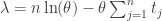
![0 = df / d\theta = {n! \over k! (n-k)!} \Bigl [ k \theta^{(k-1)} (1-\theta)^{(n-k)} - (n-k) \theta^k (1-\theta)^{(n-k-1)} \Bigr ]](https://s0.wp.com/latex.php?latex=0+%3D+df+%2F+d%5Ctheta+%3D+%7Bn%21+%5Cover+k%21+%28n-k%29%21%7D+%5CBigl+%5B+k+%5Ctheta%5E%7B%28k-1%29%7D+%281-%5Ctheta%29%5E%7B%28n-k%29%7D+-+%28n-k%29+%5Ctheta%5Ek+%281-%5Ctheta%29%5E%7B%28n-k-1%29%7D+%5CBigr+%5D&bg=ffffff&fg=333333&s=0&c=20201002)
![= \Bigl [ {k \over \theta} - {n-k \over 1-\theta} \Bigr ] f(k|\theta)](https://s0.wp.com/latex.php?latex=%3D+%5CBigl+%5B+%7Bk+%5Cover+%5Ctheta%7D+-+%7Bn-k+%5Cover+1-%5Ctheta%7D+%5CBigr+%5D+f%28k%7C%5Ctheta%29&bg=ffffff&fg=333333&s=0&c=20201002)
This will be zero when the quantity in brackets is zero, i.e., when

This equation isn’t difficult to solve for

This is the maximum likelihood estimate, or MLE, of the parameter 
As another example, suppose we expect some event (say, the decay of a radioactive nucleus) to occur at a time which is governed by the exponential distribution. Then the probability for the decay time of a single nucleus is

where 

It’s convenient to define the log-likelihood as simply the logarithm of the likelihood


Since the logarithm is a monotone function, the log-likelihood will be maximum for the same parameter value at which the likelihood is maximum. For the radioactive decay we have
The parameter value which maximizes the log-likelihood (and therefore the likelihood) is the MLE estimator, which is

so the MLE estimate of the paramter 
When a model has more than one parameter, we simply treat the parameters as a vector, and the MLE estimates are the values of that vector which give the maximum value of the likelihood function (or the log-likelihood function) for the given observed data.
In most cases, MLE estimators have some profound advantages. For one thing, the MLE estimator is a consistent estimator. This means that as the number of available data grows, the MLE estimator converges in probability to the true value of the parameter or parameters. For another thing, as the sample size grows the distribution of the MLE estimator itself approaches the Gaussian, or normal, distribution. We can even compute the asymptotic-limit variance-covariance of the parameter vector as the inverse of the Fisher Information matrix. Also, the MLE estimator is efficient, meaning that no other estimator which is asymptotically unbiased, will have lower asymptotic mean squared error. As if all that weren’t good enough, the MLE is often transformation-invariant, i.e., if 


We’ve discussed the likelihood function before, in the context of Bayesian analysis. If we multiply the likelihood function by a prior probability distribution which expresses our knowledge or belief about the parameter values before observations are made, the result is proportional to the posterior probability distribution for the parameter values. If our prior probability is uniform, then the posterior probability is proportional to the likelihood function. If we then estimate the parameters by the values which maximize the posterior probability, the estimate will be identical to the MLE estimator. Therefore in a sense the MLE estimator can be thought of as a Bayesian estimate, namely the mode of the posterior distribution when we use a uniform prior.
Because of its many advantages, because it applies to so many cases, and because it is theoretically so natural (from either a frequentist or Bayesian perspective), MLE estimation has become a workhorse for statistical analysis. In fact it’s rather common, when applying statistical models, not to worry too much about how we’ll estimate their parameters from observed data because if we can’t find a clever or simple way to do so we can always fall back on the MLE estimator (which often coincides with the clever and/or simple way). In fact many statisticians are inordinately fond of MLE as a methodology in general — and with good reason.


The advantage and disadvantage to a one room school is that you are constantly exposed to ideas which you can’t yet quite grasp. Some rise to the challenge; some sink; and some just tread water.
I appreciate the post. Thanks!
Great post.
Count me among those who are serious Likelihood fans. The assymptotic Normality of the MLEs means you can also determine confidence intervals using the chi-squared distribution with DOF equal to the number of parameters. It is intuitive, and its relation to AIC and other information criteria makes it possible to do model comparison with models of differeng complexity.
I’ve also found that it is very useful for model averaging, and that if you use Anderson and Burnhams AIC weights, it is exactly the same as taking the expectation value over all models if you start with a Uniform prior. Note that if the Prior is uninformative and roughly colocated with the central tendency of the likelihood, you get the same result.
[Response: Indeed, with a large sample the prior usually has little impact on the result anyway. Yeah, MLE is uber-cool.]
It’s a shame to respond to a serious and substantial post with an anecdotal oddity–but I can’t forbear to mention that when a buddy and I (completely quixotically/foolishly/pointlessly) did a coin-flip trial way back in high school, we actually did get one coin-flip which landed on edge. . .
[Response: That’s the first I’ve ever heard of such an event. Perhaps I’ll include the possibility in future musings.]
Well, it illustrates “real world messiness” in several senses; the trials were carried out in an extremely untidy and cluttered room, and a misdirected flip landed the coin on the edge of a rumpled cloth, which held it more or less vertical. Clearly such a result would have been far less likely in a cleaner environment!
I suppose there’s a protocol question, too; should we have just thrown that result out, instead of creating a third category in which to record it? (Which latter is what we did–with the utmost mock-seriousness.)
we actually did get one coin-flip which landed on edge. . .
Well, then you can answer a question I’ve had for almost exactly 50 years: Did you gain telepathic powers when the coin landed on edge?
This was, in fact, the premise of a Twilight Zone episode. I will date myself by saying that it’s one of my all-time favorites and that I remember quite well watching the episode’s original airing in February, 1961. (And, yes, that is Darrin from Bewitched in the photo.)
Incidentally, I believe wikipedia is wrong in saying that he “inadvertently” knocked the coin over on his way home. As I recall, it was quite intentional–Darrin had found that telepathy was not exactly an unqualified boon.
No; but perhaps the magic only works in the case of a “clean” edgestand. (See my caveat above.)
Or possibly you need to be Dick York.
That would be MUSE : Maximum Unlikelihood (and Strangeness) Estimation.
Typo in the derivative for your first example: second term should be (1-theta)^(n-k-1).
[Response: Right you are. Fixed.]
Dear Tamino
I have been grappling with MLE as part of my PhD using multinomial logit modelling. I understand it conceptually but I am still having difficulty explaining plainly it to my supervisor. So it remains an ongoing process.
This article has been of great help.
Regards Doug
Twice (in the same hallway) I missed slipping a coin into my pocket while walking down the hall. On both occasions the coins landed on edge and rolled down the hallway into wall at the end.
Invariant Bayesian estimation on manifolds:
http://projecteuclid.org/DPubS?service=UI&version=1.0&verb=Display&handle=euclid.aos/1117114330
arrives at an interesting conclusion.
David, nice article, but in my estimation it proves something that is already intuitively obvious: when you have a natural metric on a space, you will also have a natural measure (i.e., you know what the surface area or volume of a 1x1x1 co-ordinate “patch” will be: you get it from the determinant of the metric tensor); in that case, you can indeed define the MLE etc. in an invariant (or covariant) way. But this is not really different from saying that you can consistently determine air pressure in N/m^2 on the Earth’s surface, no matter what Earth surface co-ordinates you use: lat/lon, state plane, UTM, …
The real problem is when you have a parameter space which does not have a natural metric/measure: like the 1-D space of CO2 doubling sensitivity values. Then you’re lost… and this is where naively using a uniform prior can lead you astray.
Tamino, in the third paragrpah, you say “we can compute the probability of getting k flips out of n trials”, you mean “k heads”, yes? Cos each trial is going to be a flip…
[Response: Yes indeed.]
Yes, MLE is a great, as is crawling for those who haven’t yet tried walking. :) But as a mode of the posterior distribution, it is strictly speaking not translation-invariant, except for linear transformations. Sometimes models are easiest to specify as unidentifiable or almost unidentifiable – then MLE does not exist. And sometimes MLE fails by being too biased, for example with variance parameters. This leads deeper towards bayesian estimation.
Janne,
An even more important example of bias in MLE is for the shape parameter of the Weibull. However, as for the bias can be quantified. Have you looked at Weighted averaging with weights based on Likelihood? Basically, it reduces to an expectation value over the Posterior distributions if you assume a uniform Prior. I’m working on a paper that uses it, and it seems to work pretty well.
Ray, no I haven’t looked at weighted averaging. I use mostly standard MLE or MAP from standard R libraries, and then go to samplers if MLE is not enough -which enables all kinds of averages. The latter has not happened too often recently.
(It’s hard to say anything meaningful on this general level, for people’s contexts and needs seem to vary wildly. But all kinds of approximative methods exist between MLE and full bayesian, and often they should be preferred.)